← Home

Yet another flow matching tutorial

Aug 8, 2026

To understand flow matching, we need to unpack the statement below:

Flow matching learns a time-dependent vector field that transports a prior distribution (the source $p_0$) to a target distribution ($p_1$) by regressing against a tractable target vector field that is known in closed form.

The key ingredients in this statement are:

• A probability path (flow) connecting the source and target distributions
• A target vector field that generates this path
• A regression objective against this target (the loss)

Morphing probabilities

Let's say we have a simple Gaussian prior $p_0~𝒩(0,I)$, and a target distribution $p_1$ that is a mixture of two Gaussians centred at $x_1^{(1)}$ and $x_1^{(2)}$. Let's pick some points from the target distribution. Over time, we want points sampled from random noise to "turn" into those points.

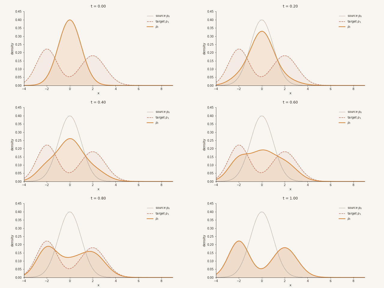
This "morphing" of the source distribution into the target distribution is the holy grail of generative modelling. If we can capture the target this way, we can do density estimation and sample new points from it as well. How is this achieved?

• In the animation below, we illustrate what a desired transformation looks like. Eight points are sampled from the prior $p_0$. For each choice of target point $x_1$, we want a transformation that collapses the entire prior into a point mass at that $x_1$. The animation shows two such transformations at once — the red one steering every noise sample toward $x_1=x_1^{(1)}$, the green one steering the same samples toward $x_1=x_1^{(2)}$. Just observe what's happening for now; we'll derive the transformation shortly.

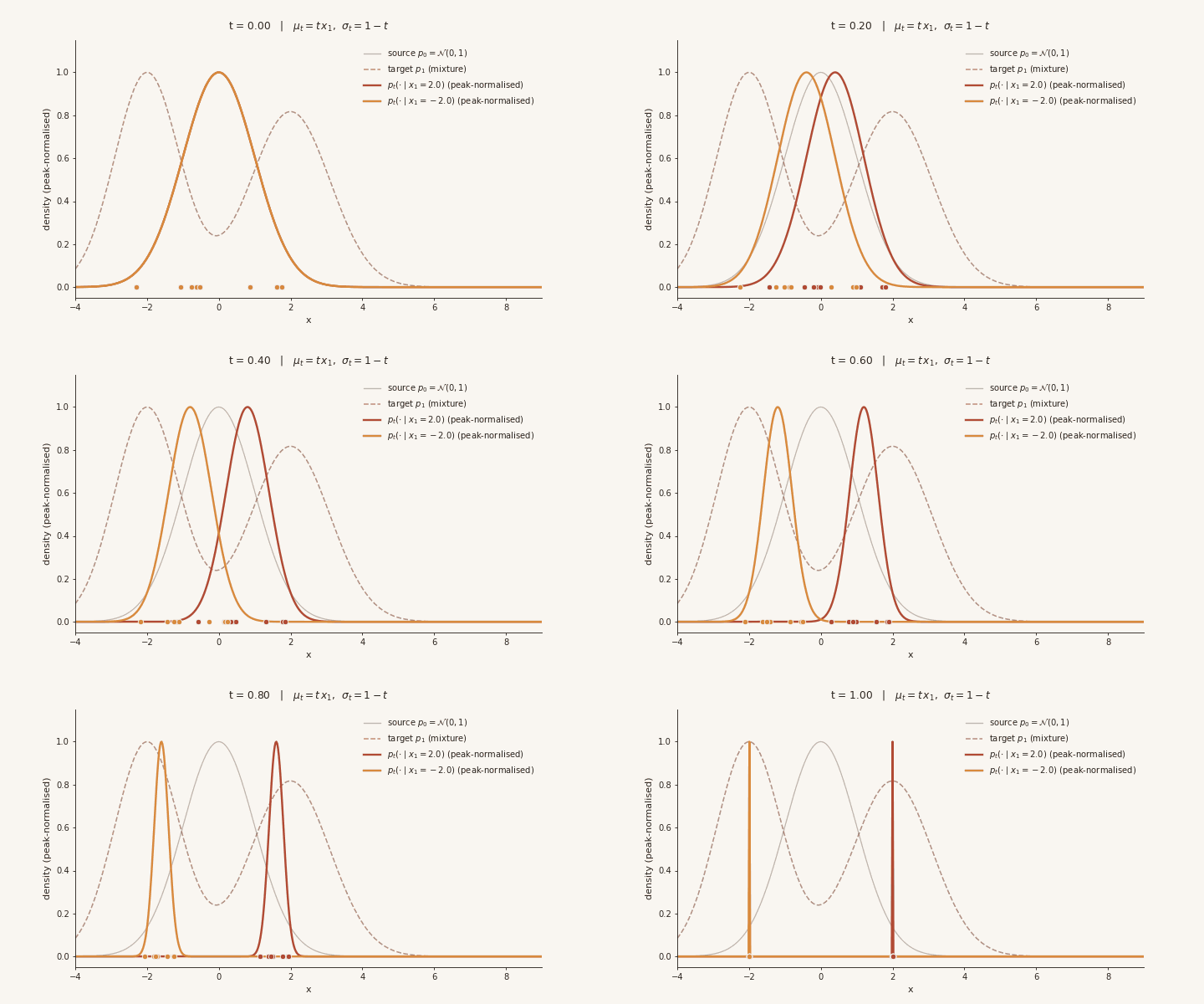
What's happening above is mathematically relatively straightforward.

• We sample a point $x_0$ from $p_0$ as defined before.
• At each time step, we transform this point in the following way:

$$x_t={\mu }_t(x_1)+{\sigma }_t(x_1)x_0$$

• This is a so-called affine transformation. It gives us a useful property:
  • If we start with a Gaussian, an affine transform of this Gaussian stays Gaussian throughout.
  • For Gaussian inputs, our sequence of transformations produces Gaussian outputs.
  • The transformation itself, viewed as a function of $x_0$, is what we call the flow map:

$${\psi }_t(x_0\mid x_1)={\mu }_t(x_1)+{\sigma }_t(x_1)x_0$$

But how can we be certain that this flow map takes us from $p_0$ to $p_1$?

To answer this, we need some notation and conceptual machinery.

The conditional probability path

We define a conditional probability path $p_t(x\mid x_1)$, the probability path of a source point through time conditioned on a single sampled target point $x_1$. We sample $x_0$ from our source distribution and apply the flow map at every time step. Since $x_0$ is Gaussian and the flow map is affine, $p_t(x\mid x_1)$ is Gaussian at every $t$ — so the conditional probability path is a path of Gaussian conditionals.

First, let's visualise three sample paths for three sampled points from the target distribution. Remember that each path $p_t(x\mid x_1)$ is Gaussian, and in the final time step the path collapses onto the point $x_1$.

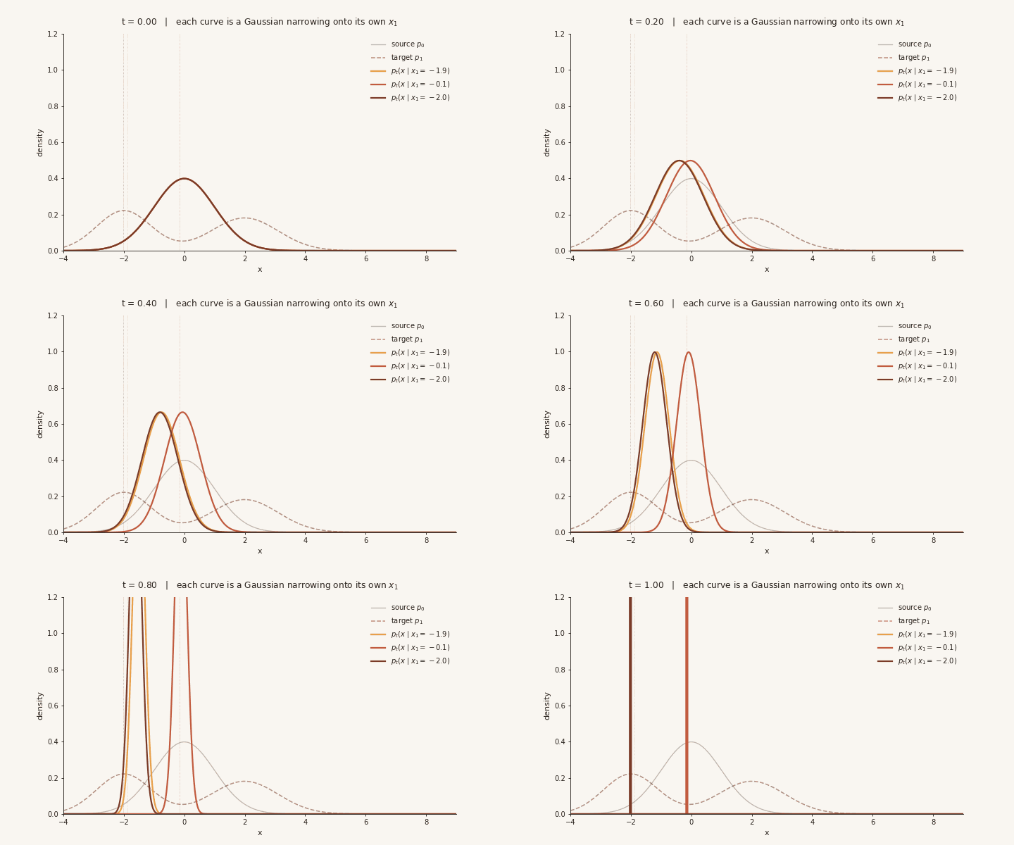
We had three target points above for $x_1$. Generally, the marginal probability path is:

$$p_t(x)=\int p_t(x\mid x_1)q(x_1)d{x}_1\approx \frac{1}{M}{\sum }_{i=1}^M{p}_t(x\mid x_1^i)$$

assuming we sample $M$ points $x_1^i~q$.

Let's visualize the marginal probability path as well with the conditions, showing how the stacked histograms evolve over time for the sampled points.

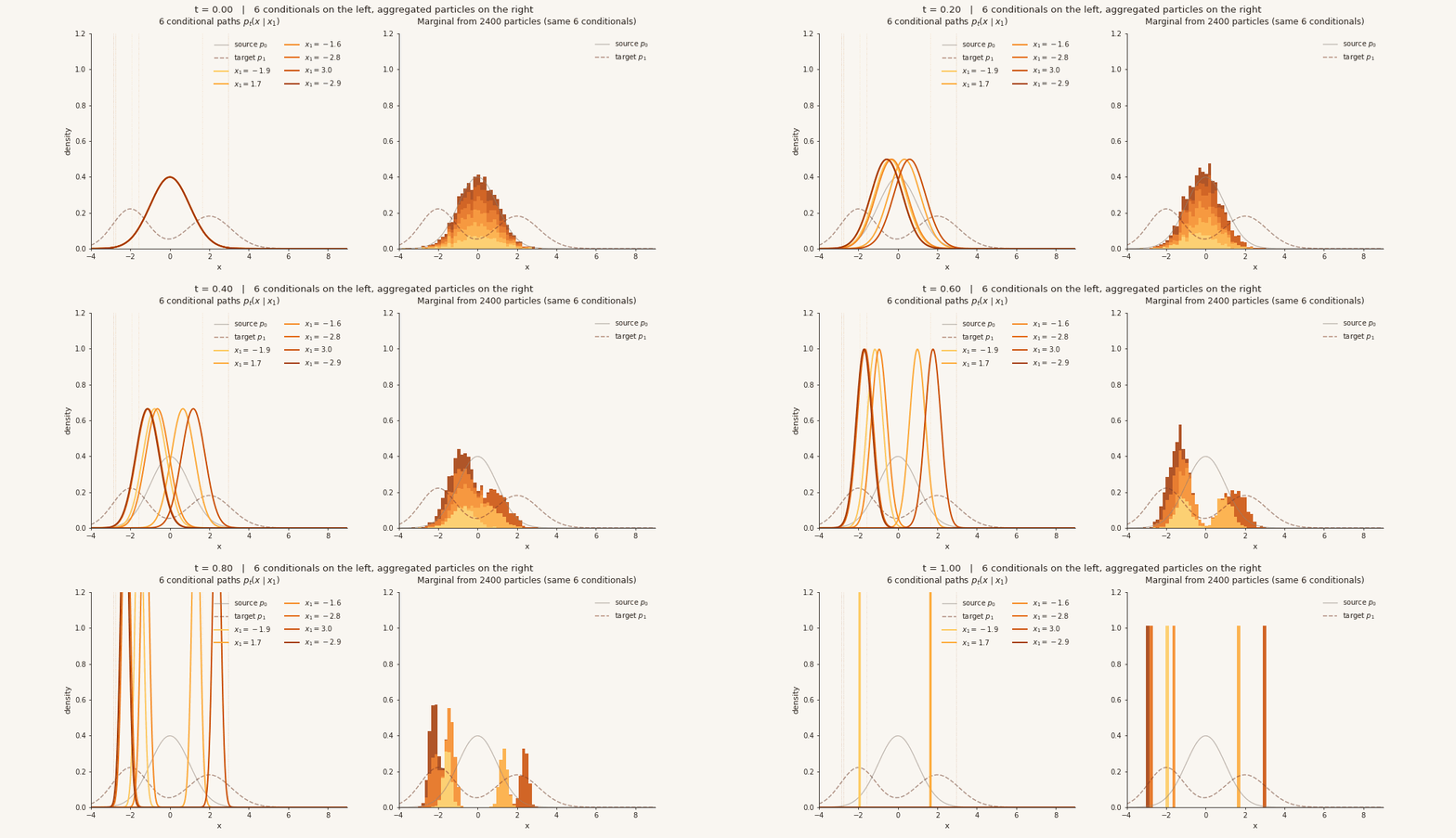
See how the probability mass concentrates (the "delta function") around the target points at the final time step. This is what we want!

In summary, the important equations are:

$$x_t={\mu }_t(x_1)+{\sigma }_t(x_1)x_0$$ $$p_t(x\mid x_1)=𝒩(x\mid {\mu }_t(x_1),{\sigma }_t(x_1{)}^{2}I)$$ $$p_t(x)=\int p_t(x\mid x_1)q(x_1)d{x}_1\approx \frac{1}{M}{\sum }_{i=1}^M{p}_t(x\mid x_1^i)$$

• The first defines how every point sampled from $p_0$ is transported toward $x_1$ (the conditional flow).
• The second defines the conditional probability path for each sampled $x_1$ — a Gaussian with a mean and variance at every step $t$ set by the schedule.
• The third defines the marginal probability path, obtained by averaging the conditionals over $q(x_1)$.

Flow Matching

We are ready to introduce flow matching [1].

• Given a flow map ${\psi }_t(x_0\mid x_1)$ that, as $t$ goes from $0$ to $1$, pushes a noise distribution $p_0(x)$ toward the target $p_1(x)$, we can derive the conditional vector field that generates the conditional probability path:

$$\frac{d}{dt}{\psi }_t(x_0\mid x_1)=u_t({\psi }_t(x_0\mid x_1)|x_1)$$

• We can learn a marginal vector field $v_t^{\theta }$ through the following regression (the conditional flow matching objective):

$${ℒ}_{\mathrm{C}\mathrm{F}\mathrm{M}}(\theta )={𝔼}_{t,x_1~q,x_0~p_0}{\Vert v_t^{\theta }({\psi }_t(x_0\mid x_1))-\frac{d}{dt}{\psi }_t(x_0\mid x_1)\Vert }^2$$

where $v_t^{\theta }(·)$ is a neural network taking $x$ and $t$ as input.

Why does this work at all?

Here are the key contributions of the flow matching paper:

• Equation 8: Defining the marginal velocity field through marginalizing over the conditional vector fields and the posterior of the conditional probability path.
• Theorem 1: If the marginal velocity field is defined via Equation 8, we can say that the marginal velocity field generates the marginal probability path ($p_t(x)$), which is exactly we want! Without this result, it would not be clear at all that we can make use of the conditionals in our model.
• Theorem 2: This shows that the gradients of the flow matching objective are equal (losses up to a constant) if we were to use the conditional velocity field in the flow matching objective. Without this theorem, it would not be possible to train the model, since the marginal field cannot be computed.
• Theorem 3: Constructs a flow map whose time-dependent derivative is the conditional velocity field, and this velocity field generates the required Gaussian conditional probability path.

This is how the flow-matching objective sidesteps the discontents of computing the marginal distribution. Without these results, we would not be able to verify that our resultant (conditional) probability paths are correct, and learning the field indeed generates this path.

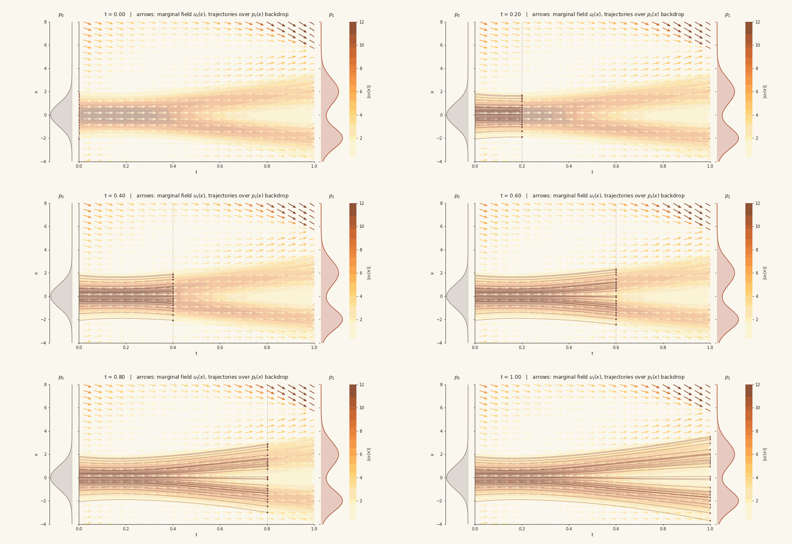
The presence and absence of straight lines

One interesting thing to observe here is that, although our conditional path is defined by a linear interpolant (the affine flow map), the marginal field that generates the marginal path is not, in general, straight for each point sampled from $p_0$ and transported to $p_1$. Why is this the case?

• At each $(x,t)$, the conditional velocity field is $u_t(x\mid x_1)={\displaystyle \frac{x_1-x}{1-t}}$.
• Many different $x_1$ can be reached from the same $(x,t)$, each inducing a different conditional arrow.
• The marginal velocity field at $(x,t)$ is the weighted average of these conditional arrows, with weights given by the posterior $p(x_1\mid x,t)$.
• If the arrows were all weighted equally, the average would collapse back into a single conditional arrow aimed at the mean $x_1$, and the resulting trajectory would be a straight line.

But that's the key point — the weights are not equal, and they shift as $(x,t)$ changes. This is a subtle point that the flow matching paper does not emphasise.

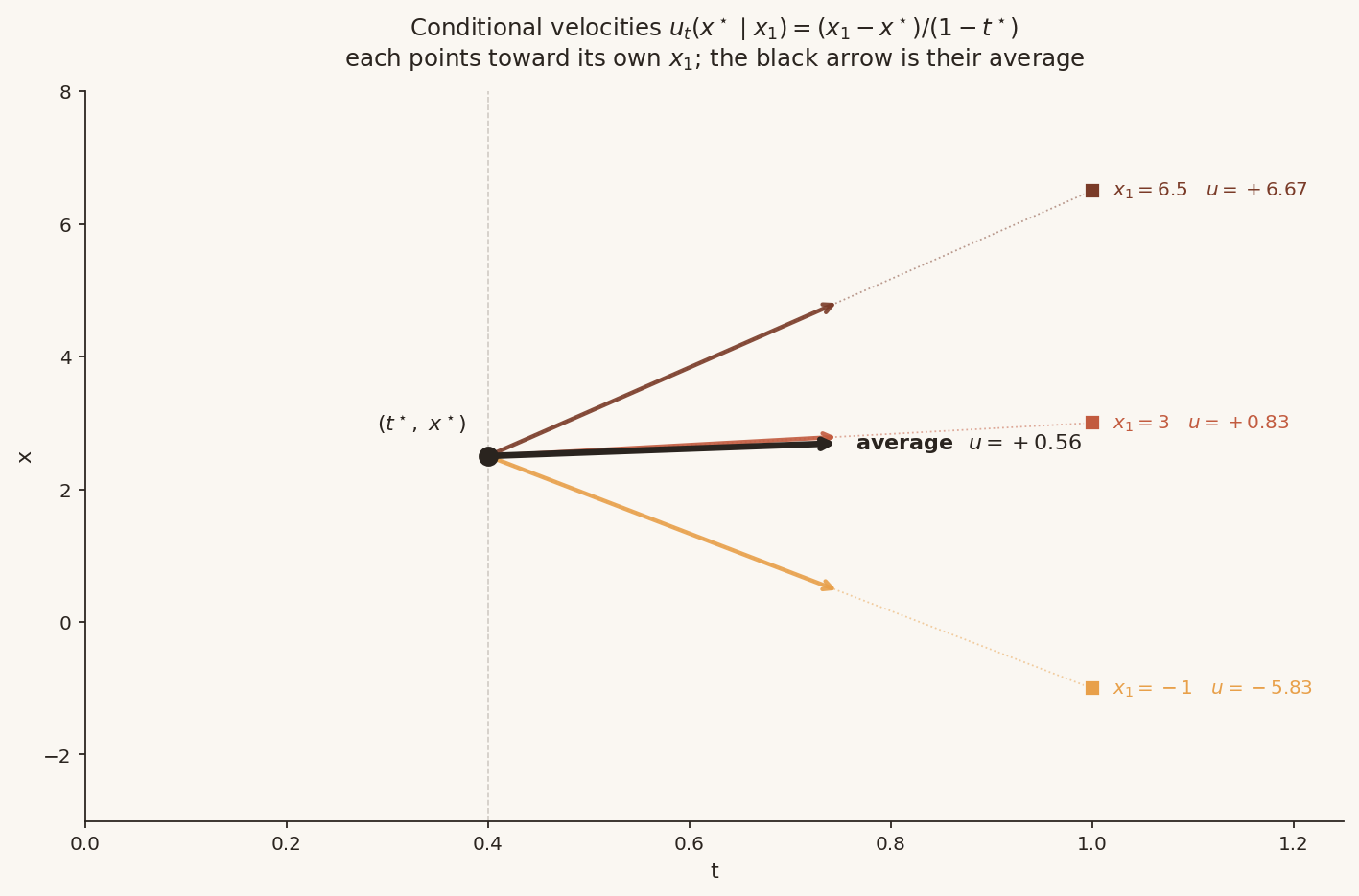
Let's say we sample three points from our known target mixture:

$x_1^{(i)}\in \{[6.5,3.0,-1.0]\}$

At $(x^{\star },t^{\star })=(2.5,0.4)$, the three conditional velocities are ${\left\{v^{(i)}\right\}}_{i=1}^3=[6.67,0.83,-5.83]$: one arrow pointing strongly up, one slightly up, and one strongly down.

With equal weights, the averaged (marginal) velocity is just the arithmetic mean: $u_t(x)\approx 0.56$.

If we did this at every $(x,t)$, we would get piecewise straight trajectories, and the resulting path from each $x_0$ would be a straight line.

But is each $x_1$ really weighted equally?

Let's look at how the marginal velocity field is actually defined:

$$u_t(x)=\int u_t(x\mid x_1)p(x_1\mid x,t)d{x}_1$$

No! The weights are the posterior $p(x_1\mid x,t)$, which depends on the target distribution (in our toy example, a mixture of two Gaussians). We use Bayes' rule to compute it:

$$p(x_1\mid x,t)=\frac{p_t(x\mid x_1)p(x_1)}{p_t(x)}$$

• $p_t(x\mid x_1)$ is defined by us in closed form from earlier.
• $p(x_1)$ is the target distribution, here a mixture of two Gaussians (known in closed form).
• $p_t(x)=\int p_t(x\mid x_1)p(x_1)d{x}_1$ is the marginal. For our toy example, where $p(x_1)$ is known in closed form, we can compute this integral.

So in this toy setting, $p(x_1\mid x,t)$ can be computed pointwise for all $x_1$, and the weights are available directly.

In general, however, $p_t(x)$ is intractable because we typically have only samples from $p(x_1)$, not a closed-form density, so the integral above cannot be evaluated. Posterior sampling techniques (e.g. MCMC) can approximate it, but they are prohibitively expensive — and avoiding this is exactly what flow matching is designed to do.

In our case, since we assume we know $p(x_1)$ in closed form, we can compute the posterior directly.

It is this posterior that gives rise to the "bending" phenomenon we see below.

We provide a worked example below.

Take $x_1^{(i)}\in \{[6.5,3.0,-1.0]\}$ at $(x^{\star },t^{\star })=(2.5,0.4)$, so $1-t^{\star }=0.6$.

The conditional velocities $u_{t^{\star }}(x^{\star }\mid x_1)=(x_1-x^{\star })/(1-t^{\star })$ are:

• $x_1=6.5$: $(6.5-2.5)/0.6\approx 6.67$ (strongly upward)
• $x_1=3.0$: $(3.0-2.5)/0.6\approx 0.83$ (gently upward)
• $x_1=-1.0$: $(-1.0-2.5)/0.6\approx -5.83$ (strongly downward)

Three arrows pointing in very different directions.

With equal weights, the averaged velocity is the arithmetic mean:

$$u_{t^{\star }}(x^{\star })=\frac{1}{3}(6.67+0.83-5.83)\approx 0.56$$

A small positive number. And this is just the conditional velocity aimed at ${\overline{x}}_1=(6.5+3.0-1.0)/3\approx 2.83$:

$$\frac{{\overline{x}}_1-x^{\star }}{1-t^{\star }}=\frac{2.83-2.5}{0.6}\approx 0.56$$

Same answer. Equal-weight averaging collapses the three-arrow average back into a single conditional field aimed at one fixed target ${\overline{x}}_1$ — and conditional fields are straight lines. So if we used equal weights everywhere, the trajectory would be a straight line from $x_0$ to ${\overline{x}}_1$. No bending.

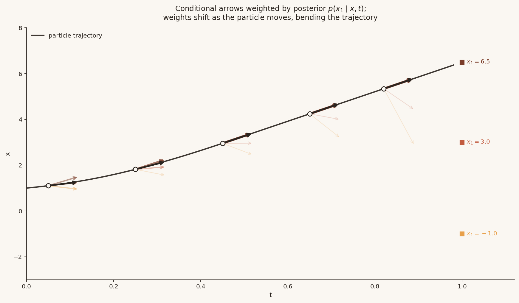
With posterior weights, the weights are given by Bayes' rule:

$$p(x_1\mid x^{\star },t^{\star })\propto 𝒩(x^{\star };t^{\star }{x}_1,(1-t^{\star }{)}^2)p(x_1)$$

Computing the (unnormalised) Gaussian likelihood for each sample at $(x^{\star },t^{\star })$:

• $x_1=6.5$: residual $2.5-0.4·6.5=-0.1$, exponent $-(-0.1{)}^2/(2·0.36)\approx -0.014$, likelihood $\approx 0.986$
• $x_1=3.0$: residual $2.5-1.2=1.3$, exponent $-(1.3{)}^2/0.72\approx -2.35$, likelihood $\approx 0.096$
• $x_1=-1.0$: residual $2.5+0.4=2.9$, exponent $-(2.9{)}^2/0.72\approx -11.7$, likelihood $\approx 8\times {10}^{-6}$

(Taking a uniform prior over the three points, so $p(x_1)$ contributes a constant factor that cancels in normalisation.)

Normalising across the three:

$${\left\{w^{(i)}\right\}}_{i=1}^3\in \{[0.911,0.089,0]\}$$

The first sample dominates because its conditional mean $x_1=2.6$ lands almost exactly on $x^{\star }=2.5$ — it's the most plausible target given where we are at time step $t^{\star }$.

Posterior-weighted marginal velocity:

$$u_{t^{\star }}(x^{\star })=0.911·6.67+0.089·0.83+0·(-5.83)\approx 6.15$$

Comparing with the equal-weight answer of $0.56$, we get the same three conditional arrows but a completely different average — because the weights are no longer uniform, they reflect which target is most consistent with the current position.

Crucially, those weights are different at a different $(x,t)$, so the next step of the trajectory will average the same three arrows differently. That shifting weight is what bends the path.

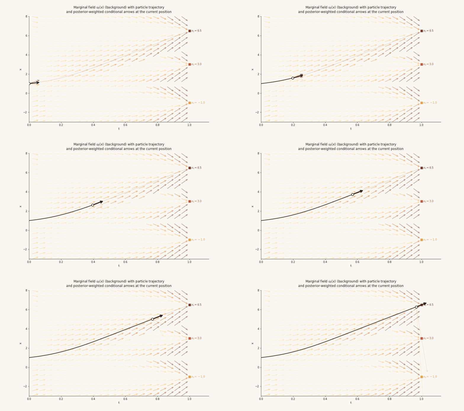
The animation above clarifies the important concept — the conditional paths defined by our flow map are all straight lines, but the marginal velocity field generates curved trajectories. Remember this point; it matters later.

Learning the velocity field for an unknown data distribution

Until now, we have worked with a simple mixture of Gaussians. While the analytic form of every object of interest was available — including the posterior — this is not a "realistic" setting. We assumed closed-form access to $p(x_1)$ so that we could illustrate the important concepts in the paper.

In this section, we finally use flow matching for what it is useful for in the first place — generative modelling by estimating an unknown distribution. For this, we use the moons dataset.

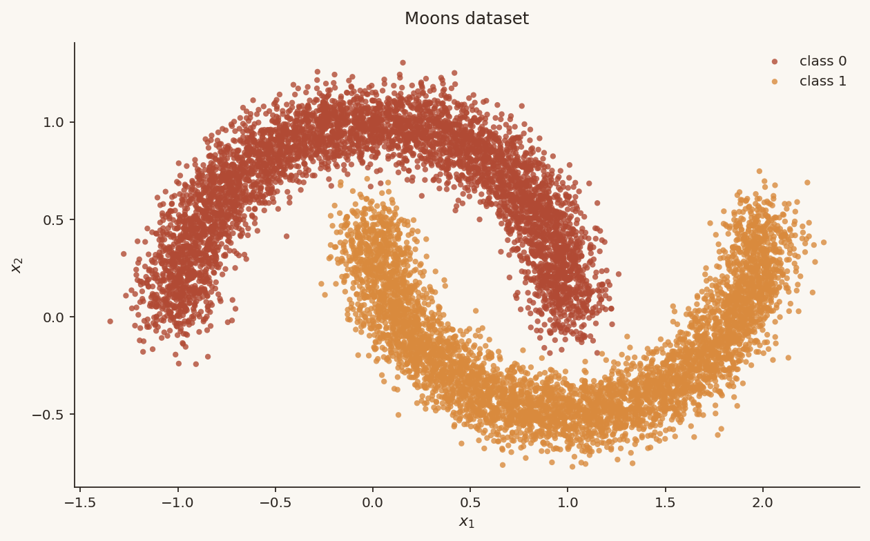
Training

• We learn the underlying conditional vector field using a neural network.
• The inputs to this network would be the input to the vector field: the position $x$ and time step $t$.
• At each step, sample the source and target points, sample a time step
• Use the flow map formula to determine where we land up ($x$) at time $t$
• Compute the velocity field using $x$ and $t$
• Regress against the known velocity field
• Compute loss
• Backprop
• Repeat!

Architecture

A simple 3-layer MLP with the ReLU activation function will be enough for this task. It will take approximately ~30s to train on the CPU.

Generation (Sampling)

Having learned the underlying vector field, we can now sample new points from the target. How?

By solving a simple ordinary differential equation. Start with the prior (noise), and follow the learned velocity field from time $t:0\to 1$. That's it!

$$x_{i+1}=x_i+v_{\theta }(x_i,t_i)·\Delta t,x_0~𝒩(0,I)$$

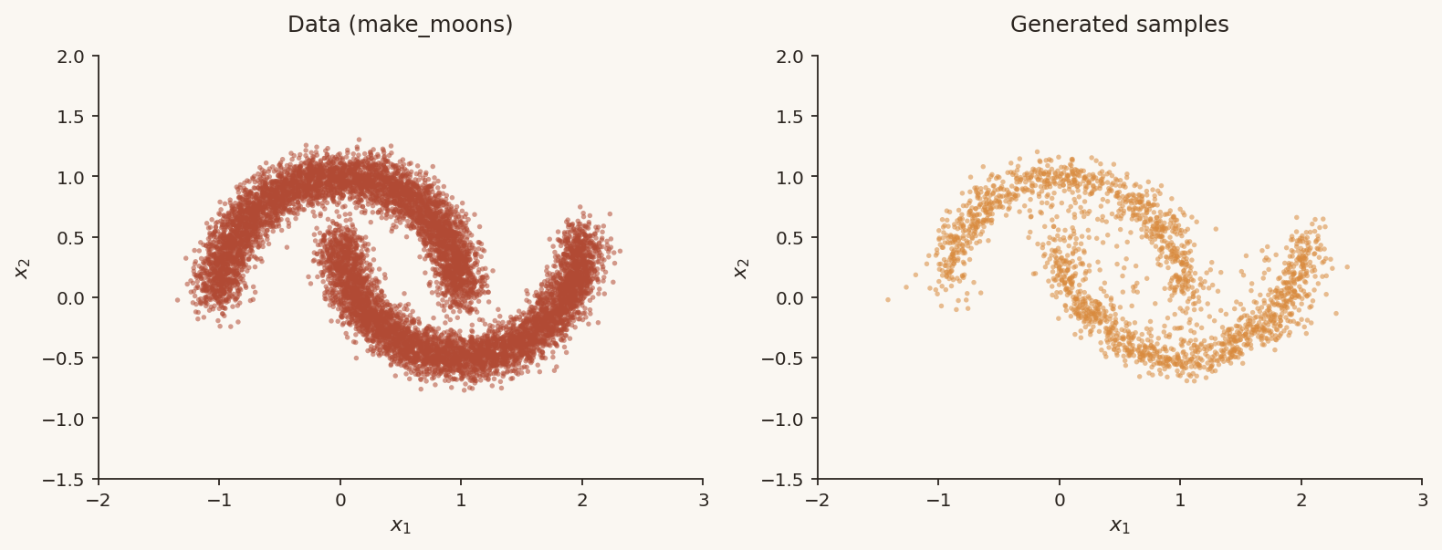
Since we compute the position at each time step, we can also visualize how nicely the original data morphs into a shape we are familiar with by now.

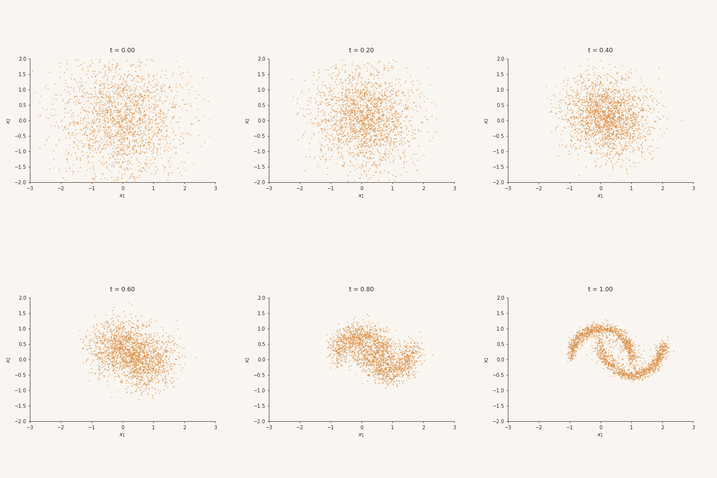
Epilogue

Flow matching has turned out to be one of the most impactful techniques for density estimation and generative modelling in recent times. They are conceptually elegant, mathematically sound, and implementation is simple. However, there are caveats:

• There is a fixed assumption here about the source distribution: we took it to be a standard Gaussian.
• Many cells ago, we observed: "the conditional paths defined by our flow map are all straight lines, but the marginal velocity field generates curved trajectories."
• Why is this an issue? The learned curved marginal field leads to expensive sampling at inference time, because the ODE solver needs more steps to reach the endpoint.

These two questions motivated several improvements since the Flow Matching paper appeared. In particular, learning a velocity field that leads to straight marginal flows, and relaxing the Gaussian assumption on the source distribution, became active areas of enquiry.

The Rectified Flow work [2], for instance, introduces a reflow procedure: given a trained flow, one re-pairs $x_0$ and $x_1$ by running the learned ODE, then retrains on these deterministic couplings. Iterating this procedure progressively straightens the marginal trajectories and, in the limit, yields a coupling that solves (an entropically regularised version of) an optimal transport problem. The key intuition is that after reflow, trajectories no longer cross: at each $(x,t)$, essentially only one path passes through, so the repeated re-averaging over shifting posterior weights — which produced the bending we observed above — is largely eliminated.

From the paper, here is an intuitive sentence:

"We can view the linear interpolation $X_t$ as building roads (or tunnels) to connect (the coupling) ${\pi }_0$ and ${\pi }_1$, and the rectified flow as traffics of particles passing through the roads in a myopic, memoryless, non-crossing way, which allows them to ignore the global path information of how $X_0$ and $X_1$ are paired, and rebuild a more deterministic pairing of $(Z_0,Z_1)$."

A nice work that unifies this couple-run-optimal-transport view is presented in [3]. It also presents a framework that goes beyond independent coupling of $(X_0,X_1)$, to a joint coupling through the optimal transport map defined by the 2-Wasserstein distance.

This work also presents an elegant generalisation of the optimal transport view in conditional flow matching to arbitrary source distributions, called the Schrödinger Bridge Conditional Flow Matching (SB-CFM).

Finally, there has been a lot of work introducing analogous unifications in the discrete data setting [4, 5], such as language. Remember, everything we discussed here was in the continuous-time formulation, and flow matching is indeed a continuous normalising flow (CNF) [6] trained in a better way through a better objective.

References

[1] Lipman, Yaron, et al. "Flow matching for generative modeling." arXiv preprint arXiv:2210.02747 (2022).

[2] Liu, Xingchao, Chengyue Gong, and Qiang Liu. "Flow straight and fast: Learning to generate and transfer data with rectified flow." arXiv preprint arXiv:2209.03003 (2022).

[3] Tong, Alexander, et al. "Improving and generalizing flow-based generative models with minibatch optimal transport." arXiv preprint arXiv:2302.00482 (2023).

[4] Campbell, Andrew, et al. "Generative flows on discrete state-spaces: Enabling multimodal flows with applications to protein co-design." arXiv preprint arXiv:2402.04997 (2024).

[5] Gat, Itai, et al. "Discrete flow matching." Advances in Neural Information Processing Systems 37 (2024): 133345-133385.

[6] Chen, Ricky TQ, et al. "Neural ordinary differential equations." Advances in neural information processing systems 31 (2018).